Introduction

I want to simulate a tree in motion, being blown by the wind, or something like that.

I will model the tree as a set of rigid bodies, coupled (in a tree topology, of course) by rotary spring+damper joints.

Nomenclature

Take a look at the free-body diagram in figure 1. This is a simple mechanical linkage of two tree limbs, \(A\) and \(B\). I use the convention that \(A\) is the parent limb (closer to the root of the tree) and \(B\) is the child limb. You could imagine how to make this more complicated:

• add more children to the end of \(A\), so that \(B\) has some siblings.

• add children to the end of \(B\), so that \(A\) has grandkids.

• both of the above.

But to derive equations of motion, we can just stick with \(A\) and \(B\) and generalize later.

Each limb (generically named \(F\)) has two dynamic properties of interest: \(\boldsymbol{C}_{IF} \in \mathrm{SO}(3)\), the direction cosine matrix relating its orientation to an inertial frame, and \(\boldsymbol{\omega}_{F}^{IF} \in \mathbb{R}^3\), the angular rate of the limb \(F\) with respect to the inertial frame. You can see this in figure 1.

Each limb has additional static properties:

• Inertia, \(\boldsymbol{I}_F \in \mathbb{R}^{3\times 3}\).

• The direction the limb points in its local coordinate system, \(\boldsymbol{u}_F \in \mathbb{R}^{3}\).

• The length of the limb, \(L_F\).

• The stiffness (Hookean) coupling the element to its parent, \(k_F\).

• The damping coefficient coupling the element to its parent, \(c_F\).

The limb \(F\) has one more property, important for defining its dynamics: the rest orientation \(\boldsymbol{C}_{If}\). The lowercase version of the limb’s letter is used to indicate the rest frame of the limb, e.g. \(f\) is the rest frame of \(F\). This is the orientation of the element (with respect to its parent) which exerts zero restoring torque. This is the analog of the natural length of a linear spring.

So when the dynamic attitude of both \(A\) and \(B\) match their rest attitudes, i.e. when \(\boldsymbol{C}_{IA} = \boldsymbol{C}_{Ia}\) and \(\boldsymbol{C}_{IB} = \boldsymbol{C}_{Ib}\), there will be zero restoring moment between the two.

Some additional bits of notation for later:

• \((\bullet)^\times: \mathbb{R}^3 \rightarrow \mathfrak{so}(3)\) is the “cross” operator, taking vectors into a skew-symmetric matrix that can be used for computing cross products, e.g. \(\boldsymbol{u}^\times\boldsymbol{v} \equiv \boldsymbol{u} \times \boldsymbol{v}\) for \(\boldsymbol{u}, \boldsymbol{v} \in \mathbb{R}^3\).

• \((\bullet)^\vee: \mathfrak{so}(3) \rightarrow \mathbb{R}^3\) is the “uncross” operator, taking the elements of a skew-symmetric matrix and putting them back into a vector, i.e. \((\boldsymbol{u}^{\times})^\vee \equiv \boldsymbol{u}\).

• \(\boldsymbol{1}\) is the identity matrix (we are using \(\boldsymbol{I}\) for inertia).

• \(\mathcal{P}(F)\) will return the parent limb of limb \(F\) in the tree.

Dynamics

The equations of motion of this tree system relate the angular accelerations of each limb to the moments applied on each limb by its parent and children. Define the dynamic state of the tree system for each limb \(F\) as \[\boldsymbol{x}^F(t) = (\boldsymbol{C}_{IF}, \boldsymbol{\omega}_F^{IF} ), \ \forall F\in \mathcal{F}\] where \(\mathcal{F}\) is the set of all limbs in the tree.

Each element of the state has a separate dynamic equation governing its time evolution. The attitude state evolves via the kinematic relationship between attitude and angular velocity: \[\dot{\boldsymbol{C}}_{IF} = -\boldsymbol{\omega}_{F}^{IF^\times}\boldsymbol{C}_{IF} \label{eqn:att-dynamics}\]

The angular velocity state evolves under Euler’s equation for rigid bodies: \[\dot{\boldsymbol{\omega}}_F^{IF} = \boldsymbol{I}_F^{-1}\Big(\big(\sum_i \boldsymbol{M}_i^F\big) - \boldsymbol{\omega}_F^{IF^\times}\boldsymbol{I}_F\boldsymbol{\omega}_F^{IF}\Big) \label{eqn:ang-dynamics}\]

The current state gives you \(\boldsymbol{\omega}_F^{IF}\), the limb \(F\) gives you its inertia \(\boldsymbol{I}_F\), so all that remains is to figure out all the moments \(\boldsymbol{M}^F_i\) on the limb. Once we have those, we can just plug equations [eqn:att-dynamics] and [eqn:ang-dynamics] into some numerical integrator and we have a dynamic state history for the tree.

There are four contributions to moments on limb \(F\)—the damping moment between \(F\) and its parent, the damping moments between \(F\) and all its children, the restoring (Hookean) moment between \(F\) and its parent, and the restoring moment between \(F\) and all its children. The next sections will explain each.

The restoring moments on a limb

The restoring moment between two elements depends on the error attitude between the two, defined as: \[\boldsymbol{E} \equiv \underbrace{\boldsymbol{C}_{Ib}^\mathsf{T}\boldsymbol{C}_{Ia} \boldsymbol{C}_{IA}^\mathsf{T}}_{\boldsymbol{C}_{ba}\boldsymbol{C}_{AI}} \boldsymbol{C}_{IB}\]

Intuitively, the definition of \(\boldsymbol{E}\) takes the relative rest orientation, \(\boldsymbol{C}_{ba} = \boldsymbol{C}_{Ib}^\mathsf{T}\boldsymbol{C}_{Ia}\), transforms it by the current orientation of \(A\), \(\boldsymbol{C}_{IA}\), and compares that to the current orientation of \(B\). In other words, we ask how \(B\) and \(A\) are aligned at rest, then imagine a \(B\) which has that alignment to \(A\) in the current absolute orientation of \(A\).

Aside on the axis-angle attitude parameterization

Any rotation can be described by a unit axis of rotation, \(\boldsymbol{a}\), and an angle about that axis, \(\phi\). Sometimes these are multiplied together and written \(\phi\boldsymbol{a}\). In an extraordinary occasion of good luck, the restoring moment between two limbs, which seeks to align some orientation with a rest orientation, is proportional to the same axis-angle expression: \(\phi\boldsymbol{a}\).
Intuitively, \(\boldsymbol{a}\) gives the moment direction, and \(\phi\) scales the moment, proportional to the angular offset of the two frames. All that remains is to multiply by the spring constant, \(k\): \[\boldsymbol{M}^k = -k\phi\boldsymbol{a}\]

Now, how to find \(\phi\boldsymbol{a}\) given a DCM \(\boldsymbol{C}_{IB}\)? Like this: \[\phi\boldsymbol{a} = (\boldsymbol{C}_{IB} - \boldsymbol{C}_{IB}^\mathsf{T})^\vee\]

This gives us a straightforward way to compute restoring moments on limbs, given their offset from some rest orientation. Now we can put that together with what we know about \(\boldsymbol{E}\).

Given \(\boldsymbol{E}\), the restoring moment on \(B\) is simply the axis-angle form of \(E\), multiplied by the spring constant: \[\boldsymbol{M}_B^{A,k} = -k_B(\boldsymbol{E} - \boldsymbol{E}^\mathsf{T})^\vee\]

Note that this definition holds regardless of whether \(A\) or \(B\) is actually closer to the root of the tree. \(A\) will apply a moment on \(B\) and vice versa, through the spring linking the two. The only difference: whichever limb is the parent will have additional contributions from other child limbs, whereas each child limb only has one moment contribution from their parent. (This is as if each child branch got their own spring in a joint to their parent, but no springs to their siblings. Could use some refinement).

The damping moments on a limb

On the parent side of the limb, the damping force simply counteracts the angular velocity of the limb: \[\boldsymbol{M}_B^{A,c} = -c_B\boldsymbol{\omega}_B^{IB}\]

That seems simple enough. I feel maybe there should be a differencing with respect to the parent limb’s velocity here? Or a cross product? TBR.

Drawing

To draw the tree at some point in time, pick a root point to start the tree at. Then we can recursively walk through the tree, visiting parent nodes before children, and draw lines for each branch that are oriented along the direction given by a child’s current DCM. This is a depth-first traversal of the tree.

Each branch is drawn as a start point and end point. Call these \(\boldsymbol{r}_A\) and \(\boldsymbol{r}_B\) respectively for a given branch. Then \(\boldsymbol{r}_B\) is given in terms of \(\boldsymbol{r}_A\): \[\boldsymbol{r}_B = \boldsymbol{r}_A + L_A\boldsymbol{C}_{IA}\boldsymbol{u}_A\]

Writing it up

I have this written up in Julia.

If you want to try it out, do this from the Julia REPL:

] add TreeDynamics

Then you can do

include("examples/animate.jl")

main()

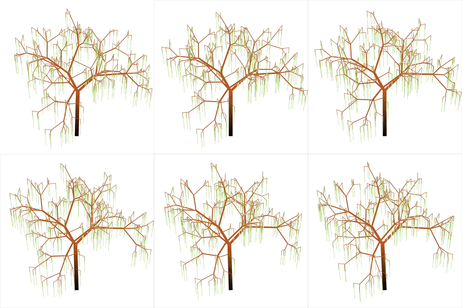
You should see a visualization along these lines:

The AbstractTrees interface in Julia was really helpful for doing this. You need to define a few functions that AbstractTrees wants you to define on your own concrete type. These are things like getters for child nodes and parent nodes. Then you can use all the breadth-first/depth-first traversal functions that AbstractTrees provides for free.¹